Part II: Simulating EEG sources
Back to Simulating and estimating EEG sources
By now our head model should be fully operational so we can start placing artificial EEG sources within the brain volume. An EEG source is just one or more source grid locations having a common temporal activation pattern. From a neurophysiological perspective, you can intuitively understand an EEG source as a compact cluster of neurons whose activity is well represented by their average post-synaptic potentials. The time course of such average post-synaptic potentials is what we call the temporal activation of the EEG source.
Simulated EEG sources
Adding new EEG sources
Let's start with the command:
myHead = add_source(myHead);
which will create a dipole of random location and orientation.
The characteristics of the dipole are stored in property Source of the
myHead object. In my case, the characteristics of the random dipole are:
>> myHead.Source
ans =

       name: []
   strength: 23.1095
orientation: [-0.6523 -0.5037 0.5664]
      angle: 47.4691
        pnt: 146
   momentum: [-15.0739 -11.6402 13.0895]
 activation: 1
      depth: 35
The information above tells us that our dipole is located at the coordinates
myHead.SourceSpace.pnt(146,:). It also tells us the orientation of the
dipole (a unit length vector) and its strength (the length of the dipole).
The result of multiplying the strength with the orientation vector is what
is called the dipole momentum. The activation of the dipole is its time
course. In this tutorial we will deal only with fixed dipoles (without temporal
variation of their time course). In the next tutorial
we will pay full attention to such a crucial feature of an EEG source.
The method add_source that we used to generate our random dipole has
several optional arguments that you can use to specify the characteristics
of the dipole that you wish to incorporate to your source model. For instance,
the following command:
myHead = add_source(myHead, 'MinDepth', 1, 'MaxDepth', 30)
will generate a dipole that is at least 1 mm deep in the brain and at most
30 mm away from the closest point on the inner skull surface. Note that
the new dipole was added to our head model, i.e. the dipole that we
generated previously is still in myHead.Source. You can check how many
EEG sources your model has by inspecting property NbSources:
>> myHead.NbSources
ans =

    2
Inspecting the properties of an EEG source
Each EEG source that you add to your head model is stored in property
Source of your head.mri object. We can inspect the properties
of the last EEG source that we just generated using the command:
myHead.Source(2)
which will display:
>> myHead.Source(2)

ans =

       name: []
   strength: 1
orientation: [-0.9549 -0.1926 -0.2261]
      angle: 47.4691
        pnt: 1
   momentum: [-0.9549 -0.1926 -0.2261]
 activation: 1
      depth: 12
Removing EEG sources
To remove an EEG source use the command:
myHead = remove_source(myHead, [1 2])
where the second argument is a vector with the indices of the sources that should to be removed. The example above will remove the two sources that we have generated so far, leaving our head model empty of any EEG source.
Make your own EEG sources
Display the help of add_source using help head.mri.add_source and read
it carefully. Then try to generate dipoles with the following characteristics:
- A radial dipole that is no more than 10 mm deep.
- A tangential dipole no more than 10 mm away from the brain surface.
- A randomly oriented dipole that is 3 times stronger than the two dipoles above and that is located at least 40 mm deep inside the brain.
- A compact EEG source that consists of 15 dipoles with random orientations and with strengths varying between 1 and 2.
NOTE: After creating each source, inspect the corresponding element
of the Source property of myHead, in order to ensure that
the source has the desired properties.
Plotting EEG sources
Source location
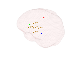
Plot the location of all four EEG sources that you generated above using the following method:
close all; % Close all existing figures
figure;    % Create a new (empty) figure
plot_source_dipoles(myHead, [1 2 3 4]);
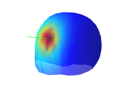
where the second input argument is a vector with indices of the EEG sources that you want to plot. The result of this command should be something similar to the first figure in the gallery below (of course the dipole locations will be different in your case, as they are random). Rotate the figure and check that the third source is indeed much deeper than the first two sources.
Source momentum
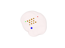
Our first attempt at plotting the EEG sources was successful but we would like to see also the orientation and the strength of each source. To plot the strength:
close all;
figure;
plot_source_dipoles(myHead, 1:4, 'time', 1, 'sizedata', 200);
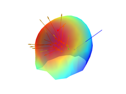
The result is shown in the second figure below. You should get something similar, but
with different dipole locations and strengths. The 'sizedata' argument
can be used to increase the default size of the source location markers. So if the size
of the dipoles markers is to small or too large in your case, try to tune the 'sizedata'
argument. In any case, the size of the dipole markers should be proportional to the dipole
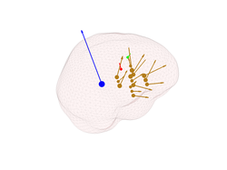
strength. If we also want to plot the orientation of the dipoles we can use:
figure;
plot_source_dipoles(myHead,[1 2 3 4],'time',1, 'sizedata',200,'momentum',10)
The 'momentum' value is analogous to argument 'sizedata' and can be used to manipulate
the length of a dipole of strength 1. So by modifying 'momentum', you will modify
the length of the dipoles arrows. But notice that, as was the case with 'sizedata',
argument 'momentum' is only for display purposes and has no effect on the properties of
the underlying dipoles. That is, the strength of the underlying dipoles is not affected
by you playing with 'momentum' or 'sizedata'.
Source leadfield
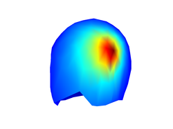
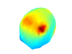
Each EEG source generates a characteristic distribution of scalp potentials. In the following I will loosely refer to such pattern as the source leadfield. The source leadfield is the _normalized potential distribution that we would see at the scalp if only the source of interest would be active and all other sources would be silent. You can plot the source leadfield with the command:
figure;
plot_source_leadfield(myHead,1)
Don't forget to use the rotate tool from the figure toolbox to visualize properly the topography of scalp potentials that is generated by the EEG source dipole.
A very important point is that the source leadfield is completely independent of the temporal activation of the source. This means that, if only one source is active, the normalized distribution of scalp potentials will be the same at any time, even if the underlying source has very complex temporal dynamics. This has also implications for localizing the source afterwards because the only thing that we need to (attempt to) localize an EEG source is its source leadfield.
You can also plot on the same figure the location and orientation of the source:
close all;
figure;
plot_source_leadfield(myHead,1, 'momentum', 50)
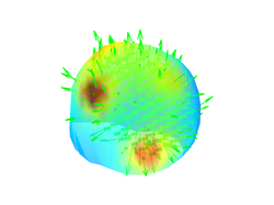
or plot that information for all EEG sources simultaneously:
close all;
figure;
plot_source_leadfield(myHead,1:4,'momentum',50)
Below you can find some of the figures that you may generate in this section of the tutorial:
Background noise
To be more realistic you can also simulate the presence of background (noisy) activity. It is difficult to define what is noisy neural activity. The easiest way is probably using an example. If you are interested in studying the generators of EEG activity in the alpha band then we would regard as noisy any neural activity that is not related to EEG-alpha.
You can generate background noise with the command:
myHead = add_source_noise(myHead, 'MaxStrength', 1);
which will create a noisy EEG source and put it in myHead.Source. You can
identify the noisy source from the rest by the fact that the noisy source
has the name 'noise':
myHead.Source(5)

ans =

           name: 'noise'
       strength: [325x1 double]
    orientation: [325x3 double]
          angle: [325x1 double]
            pnt: [1x325 double]
       momentum: [325x3 double]
     activation: [325x1 double]
You can plot the characteristics of the noisy activity using:
close all;
figure;
plot_source_leadfield(myHead,'noise','momentum',50)
You can also visualize the effect that the noisy activity has on the overall distribution of scalp potentials at the scalp:
close all;
figure;
plot_source_leadfield(myHead, 1:5)
Please familiarize yourself with methods plot_source_dipoles and
plot_source_leadfield, and ask your tutor any questions you may have before going
any further.
What now?
Now you are ready to go to Part III of this tutorial where we attempt to localize some of the EEG sources that we just simulated.
