Part III: Localizing EEG sources
Back to Simulating and estimating EEG sources
In this last part of the tutorial we will attempt to solve the EEG inverse problem. That is, given a distribution of scalp potentials we will attempt to localize the underlying EEG sources. In fact this is just one part of the inverse solution. The full solution involves also the reconstruction of the temporal activation of the underlying EEG sources. However, we will leave that for a future tutorial where our EEG sources will have time-varying activation patterns.
In this last part of the current tutorial you may use some the sources that you generated in Part II or you may as well generate new sources altogether. I will follow the latter approach. If you decide to use new sources then you should first remove the old ones (I am assuming you generated only 5 sources):
myHead = remove_source(myHead, 1:5);
Localizing a single dipole
Let's generate a radial and superficial dipole:
myHead = add_source(myHead, 'Name', 'radial', 'strength', 1, ...
    'MaxDepth', 10, 'Angle', 0)
close all;
figure;
plot_source_leadfield(myHead, 1, 'momemtum', 50)
Now let's plot the scalp potentials that we would measure in such a single dipole scenario:
figure;
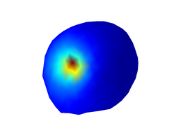
plot_scalp_potentials(myHead, 'time', 1)
The result is shown below.
As we have a single EEG source and there is no noise, the distribution of scalp potentials (what we are measuring) is identical to the leadfield generated by the only underlying EEG source (what we need for source localization). This is obviously an ideal scenario and we would expect to be able to solve the inverse problem accurately. Let's try:
myHead = inverse_solution(myHead);
figure;
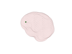
plot_inverse_solution_dipoles(myHead, 'time', 1);
The first command above will estimate the location of the source using a Minimum Norm Estimate (MNE), which is the method employed, for instance, by the MNE software. The generated figure is shown below:
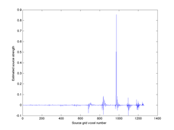
Although you can barely see it in the figure above, the inverse solver estimated non-zero (but very small) activation strengths not only at the true location of the dipole, but also at many other locations of the source grid. You can actually inspect the activation values that were estimated at each source voxel with the commands:
close all;
figure;
plot(1:myHead.NbSourceVoxels, myHead.InverseSolution.strength);
xlabel('Source grid voxel number');
ylabel('Estimated source strength');
which, in my case, looks like this:
Indeed, the only source grid location at which the strength is significantly different from zero is voxel 245, which is also the location of the true underlying dipole :
myHead.Source(1)

ans =

           name: 'radial'
       strength: 1
    orientation: [0.5630 0.8133 0.1466]
          angle: 0
            pnt: 245
       momemtum: [0.5630 0.8133 0.1466]
     activation: 1
In your case, the location of the underlying dipole is likely to be different but, if the
inverse solver did its job, then myHead.Source(1).pnt should match the location of the
maximum of myHead.InverseSolution.strength. Let your tutor know it that is not the case!
Measurement Noise
To make our simulations a bit more realistic, we will add a bit of measurement noise:
myHead = add_measurement_noise(myHead, 0.00001);
Now let's compare the source leadfield with the (noisy) measured scalp potentials:
close all;
figure;
plot_source_leadfield(myHead, 1, 'momemtum', 25);
set(gcf, 'Name', 'Source leadfield');
figure;
plot_scalp_potentials(myHead, 'time', 1);
set(gcf, 'Name', 'Measured scalp potentials');
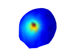
The two resulting figures are shown below:
As you can see the distribution of scalp potentials is (to the naked eye) identical to the source leadfield. Indeed the measurement noise is extremely low in our example. But let's try to localize the underlying source:
myHead = inverse_solution(myHead);
figure;
plot_inverse_solution_dipoles(myHead, 'time', 1);
figure;
plot_inverse_solution_dipoles(myHead, 'time', 1, 'exp', 4);
The latter command will use a higher weighting exponent for the plot so that stronger voxel activations will appear even stronger and weak activations will look even weaker. The resulting figures are shown below:
Let's also plot the estimated dipole strength at each source location, in a 2D plot:
close all;
figure;
plot(1:myHead.NbSourceVoxels, myHead.InverseSolution.strength);
xlabel('Source grid voxel number');
ylabel('Estimated source strength');
As you can see, the inverse estimate is completely wrong now. How is this possible, even if the scalp potentials were only marginally disturbed by noise? What would you do to try to overcome this problem?
Ill-conditioning
If you didn't guess it, the inverse estimate obtained from our noisy measurements was so poor because the leadfield matrix (i.e. the matrix of coefficients that maps current sources to potential differences at the scalp) was ill-conditioned. By ill-conditioned we mean that we cannot directly calculate an accurate pseudoinverse of the leadfield matrix. Recall from the slides on linear algebra that the pseudoinverse ''A^+'' of leadfield matrix ''A'' is defined as:
The problem here is that the term ''A^T*A'' is not invertible, due to some
columns of ''A'' being very close to linearly dependent. You can check the
conditioning of a matrix using MATLAB's command cond(). Let's check the
condition number of our leadfield matrix:
cond(myHead.SourceDipolesLeadField)

ans =

   1.2686e+16
Remember from the documentation of the cond() command that,
the larger the condition number, the worse the conditioning of the matrix
is. In our case, we obtained a very large number, clearly indicating that,
even if we still can compute the pseudoinverse, using it to recover the
source dipoles magnitudes might lead to inaccurate results, especially in
the presence of noise.
Regularization
As you learned from the course lectures, a way to deal with ill-conditioned
inverse problems is to use regularization. Method
inverse_solution() allows you to define a regularization parameter
''lambda'' to be used when computing the pseudoinverse of the leadfield:
myHead = inverse_solution(myHead, 'Lambda', 0.0001);
figure;
plot_inverse_solution_dipoles(myHead, 'time', 1);
How does the inverse solution look like now? Play around with the regularization parameter (and maybe with the level of measurement noise) and tell your tutor what you learned.
