Part I: A realistic head model
Back to Simulating and estimating EEG sources
In this tutorial we use a realistic electromagnetic model to map
intracerebral current sources (modeled as dipoles) to a set of EEG sensors.
Our model is based on a real MRI scan from an unknown subject identified
by the code 0003. Below are the main steps that we need to take in order
to build our head model. The first three steps have been already performed
for you, but you will need to carry out the other four steps to
successfully build a model that we can play around with.
Step 1: Tissue segmentation
Different brain tissues have different characteristic conductivities. A realistic head model needs to take this fact into account and, therefore, tissue types need to be segmented. Typically, only scalp, skull and cerebral tissues need to be identified in order to build a reasonably accurate electromagnetic model. However, you can complicate your model by segmenting also white and gray matter and, if you really like making your life difficult, by taking into consideration the fact that tissue conductivity (especially within white matter) is anisotropic.
In the old times, brain tissues had to be manually or semi-automatically
segmented. This was not only time consuming but also highly subjective.
Fortunately, the standardization of MRI scanning technology has
allowed the development of extremely accurate fully-automated tissue
segmentation packages. There are multiple freely available alternatives but,
arguably, the most robust and widely tested software package is
Freesurfer, developed at the Athinoula A. Martinos Center
for Biomedical Imaging.
Step 2: Surface reconstruction
Once different tissues have been identified, we need to build closed triangulated surfaces between all relevant tissue types. In our model we have three such surfaces: the outer skin surface (on which the EEG sensors rest), the outer skull surface, and the inner skull surface (within which the EEG sources may be located). These surfaces can be automatically generated using a variety of software packages. In this tutorial we used the watershed algorithm included in the MNE software, which is also maintained by the Athinoula A. Martinos Center.
The resulting surfaces are available in .tri data format in folder
db/0003:
0003-inner_skull-5120.tri
0003-inner_skull-dense.tri
...
0003-outer_skin-5120.tri
0003-outer_skin-dense.tri
There are two versions of each surface. The dense surfaces are just
more densely tessellated versions of the 5120 surfaces, which consist of
(only) 5120 vertices.
Step 3: Sensor co-localization
The purpose of having a densely tesselated outer skull surface is that
it allows for more accurate co-registration of the EEG sensor locations. That
is, it makes it easier to match each EEG sensor with a surface vertex.
For this tutorial we use a state-of-the-art sensor net with 256 sensors by
EGI. The standard sensor locations provided by EGI were co-registered
with surface 0003-outer_skull-dense.tri using Fieldtrip, and
are available in file 0003-sensors.hpts. The latter is just a text file that
you can inspect with a text editor, if you want.
Step 4: Loading and inspecting the anatomical model
You can load the surface information into MATLAB using the command:
myHead = head.mri('SubjectPath', 'db/0003')
assuming of course that you are in the tutorial_dipoles folder that you
created when you unzipped the tutorial files. The command above will
create an object of class head.mri. An object is just a convenient
representation for a bunch of data and operations (or methods) that
can be performed on that data. You can read more about
objects with MATLAB if you want.
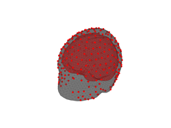
You can now easily plot the model surfaces with the command:
figure;
plot(myHead);
Just for fun, use the figure toolbox (at the top of the figure that just opened) to
rotate and zoom in/out the head model. Rotating might be slow if your computer is not
very powerful. Now, see help head.mri.plot and try to make a figure that displays
only the inner skull surface and the locations of the sensors. Then, save this figure
using MATLAB's built-in command print:
print -dpng myfigure.png
which will save the current figure in portable network graphics format in a
file called myfigure.png.
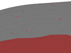
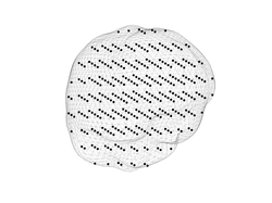
If you zoom in the head model that we generated above, you will see that the EEG sensors (displayed as red dots) do not fall exactly on vertices of the outer skin surface. Try it and you should see something like the figure on the right below.
However, recall that we said that EEG sensors need to be co-registered
with vertices of the outer skin surface. The reason for the discrepancy is that we performed the co-registration using the dense version of the outer
skin surface but our head model is actually based on a lower-resolution
triangulated surface (the 0003-outer_skull-5120.tri surface). Indeed, you
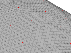
can see that the sensors do fall on vertices of the dense surface:
figure;
h = plot(myHead, 'Surface', 'OuterSkinDense');
set(h(1),'facealpha',1,'edgealpha',1);
The 'facealpha' and 'edgealpha' are just properties of the surface plot
that we can use to manipulate the transparency of the triangles (the faces) and of the edges.
You can force the sensors to really fall on vertices of the low resolution outer skin surface with the command:
close all; % Just to close previous figures
myHead = sensors_to_outer_skin(myHead)
Zoom-in the generated figure to ensure that the sensors are now placed on vertices of the coarse head surface.
Step 5: Intracerebral source grid
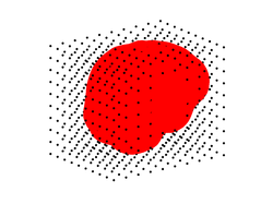
In order to build an electromagnetic model we need to specify the spatial locations where EEG sources may be located. This is typically done by uniformly sampling the inner skull volume using a regular 3D grid:
myHead = make_source_grid(myHead, 0.5)
where the second input argument is a scalar in the range [0 1] that determines the density of the generated grid. The higher the density, the higher the number of elements in the source grid. Play a bit with the density value to see how it works. However, this tutorial has been tested only with a grid density of 0.5. Using a higher or lower value might have unexpected results, like abnormally inaccurate inverse solutions, and is not recommended.
What do you think are the benefits of having a denser source grid? And the disadvantages?
Step 6: BEM computation
The steps above have fully described the anatomical aspects of our head model. It is now time to compute the electromagnetic model. That is, to describe the mapping that relates activity at the source grid locations to activity at the scalp sensor locations. This mapping can be computed using a Boundary Element Method (BEM).
Again, there are multiple freely available software packages implementing the BEM. EEGLAB, Fieldtrip, and the MNE software are just three examples. Moreover, each of these software packages include several algorithms for computing the BEM coefficients. In this tutorial we use the default algorithm (Oostendorp and Oosterom, 1989) of the Fieltrip toolbox. To compute the BEM model, just run the command:
myHead = make_bem(myHead);
The step above might take few minutes to compute.
As you may have guessed already, the computation of the BEM model will take
longer, the denser the triangulated boundaries of the head model. This is precisely
the reason why we did not use the dense surfaces to build our model, but decided to use those only for sensor co-registration purposes. An even more
important problem of using too dense surfaces is that it can lead to numerical
innaccuracies due to the fact that the model may become ill-conditioned.
Step 7: Leadfield generation
The actual mapping from source grid locations to EEG sensors (also known as the leadfield matrix) is computed, based on the BEM model, with the following command:
myHead = make_leadfield(myHead);
This step may also take a couple of minutes to compute. It will take longer the higher the number of sensors and the higher the number of source grid locations.
The result of this step is a 257x3xN matrix, where N is the number of
source grid locations. This matrix is stored in the LeadField property
of our myHead object:
myHead.LeadField % The leadfield matrix
The meaning of the leadfield matrix is straightforward. If you had a
dipole ''m=[m_x, m_y, m_z]'' at the ''i''th grid location (whose coordinates
are in myHead.SourceSpace.pnt(i,:)), then the EEG measured at the ''j''th
sensor would be:
% EEG potential measured at the 10th sensor assuming a single
% dipole at the 100th source location:
i = 100;
j = 10;
% The dipole coordinates:
m = [0;1;0]
leadField_ji = myHead.LeadField(j, :, i)
v = leadField_ji*m
There is an important point that you should realize here. The scalp potentials generated by a source dipole do not depend only on the strength of the source (the length of the dipole) but they do also strongly depend on its orientation. As you will see below, dipoles that are close to the scalp and are tangentially or radially oriented with respect to the scalp surface generate very characteristic distributions of potentials across the scalp.
NOTE: Computing the leadfield matrix requires solving Maxwell equations, under the boundary conditions imposed by the head model. These are complicated differential equations and some of you may wonder how can their solution be as simple as a linear and instantaneous mapping. The answer is that the exact solution to Maxwell equations is far from being that simple. However, in EEG and MEG applications we take advantage of the fact that the signals measured rarely exceed frequencies above 1 KHz. At such low frequencies, we can safely use the so-called quasi-static approximation of Maxwell equations, which indeed leads to a solution that is just a linear and instantaneous mapping. For those interested in bioelectromagnetism I recommend the book by (Malmivuo and Plonsey, 1995).
What now?
Now you are ready to go to Part II of this tutorial where we will use the head model that we just prepared to simulate EEG sources and to study the patterns of scalp potentials that such sources generate.
